


 20 / 23

y
(
x
) =
±
C
3
k
(
p
(
b
0
))(
x
−
b
0
)
−
3
k
−
1
(1 +
o
(1))
as
x
→
b
0
+ 0
,
and
,
at its local extremum points
,
|
y
(
x
0
)
|
=
|
b
00
−
x
0
|
−
3
k
−
1
+
o
(1)
as
x
0
→
b
00
−
0
.
Conclusion.
Note that oscillatory solutions of equations (1) and (3)
defined on
(
−∞
;
x
∗
)
or
(
x
∗
; +
∞
)
,
are the solutions of the form
y
(
x
) =
|
p
0
|
−
1
k
−
1
|
x
−
x
∗
|
−
α
h
(log
|
x
−
x
∗
|
)
, α
=
n
k
−
1
,
(18)
with
n
= 4
and
n
= 3
respectively and an oscillatory periodic function
h
:
R
→
R
.
Indeed more general result takes place. Thus, for the equation
y
(
n
)
+
p
0
|
y
|
k
−
1
y
(
x
) = 0
, n >
2
, k
∈
R
, k >
1
, p
0
6
= 0
,
(19)
the existence of oscillatory solutions of the type (18) is proved.
Theorem 5.
For any integer
n >
2
and real
k >
1
there exists a
non-constant oscillatory periodic function
h
(
s
)
such that for any
p
0
>
0
and
x
∗
∈
R
the function
y
(
x
) =
p
−
1
k
−
1
0
(
x
∗
−
x
)
−
α
h
(log(
x
∗
−
x
))
,
−∞
< x < x
∗
, α
=
n
k
−
1
,
(20)
is a solution to equation
(19).
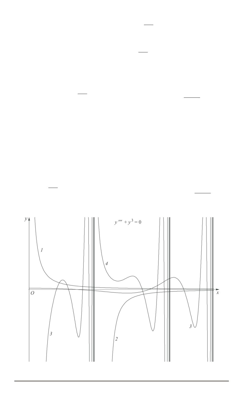
Fig. 5. Solution to equation (3)
22
ISSN 1812-3368. Вестник МГТУ им. Н.Э. Баумана. Сер. “Естественные науки”. 2015. № 2